I wanted to implement a Raspberry Pi controlled heating and hot water system. The first step in this plan would be the instrumentation of the hot water system, to give the pi the information it needed to decide when to turn the hot water on, with the following objectives.
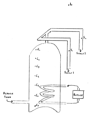
The hand drawn picture to the right attempts to show the hot water cylinder in our loft.
The Raspberry Pi used as the data logger for the ten temperature probes was fitted in the loft
To add the kernel modules required to read the DS18D20 probe temperatures to the Raspbery Pi
kernel at boot time, I added the following lines to /etc/init.d/rc.local
# Initialise the 1-wire modules
sudo modprobe w1-gpio
sudo modprobe w1-therm
Partly as it is the right place to put logging, but mostly in order to allow ramlog to
keep the temperature logging from producing many SD card writes, I created the directory
/var/log/w1_logs to contain the probe temperature readings.
Then to log the probe temperatures every five minutes I added the following crontab
0,5,10,15,20,25,30,35,40,45,50,55 * * * * /home/pi/script/w1read_corrected
after creating the file /home/pi/script/w1read_corrected containing the following script
#!/bin/bash
#

log_file=/var/log/w1_logs/w1.`date +"%Y%m%d"`
proc_file=/var/log/w1_logs/w1.processed.`date +"%Y%m%d"`
start_time=$(date +"%H:%M:%S")

if [ $(date +"%H:%M") = "00:00" ]
then
  echo "  Time   Cyld 1 Cyld 2 Cyld 3 Cyld 4 Cyld 5 Cyld 6 Cyld 7   Supp 1 Supp 2    Loft" >>$proc_file
  echo "-------- ------ ------ ------ ------ ------ ------ ------   ------ ------   ------" >>$proc_file
fi

for slave in 5d25881 5f25eb3 5f20099 5e4c468 5e643f3 5d3affe 5d3bc7c 5d39217 5e683d0 5e7209b
do
  echo Slave $slave :
  cat /sys/bus/w1/devices/28-00000$slave/w1_slave
done |tee -a $log_file | awk -v start_time="$start_time" '
  BEGIN {
    n = 0;
    slave[n] = "5d25881"; factor[n] = 1.004; delta[n] = -079.4; temp[n] = 0; n++;
    slave[n] = "5f25eb3"; factor[n] = 1.021; delta[n] = -349.7; temp[n] = 0; n++;
    slave[n] = "5f20099"; factor[n] = 0.998; delta[n] = +036.5; temp[n] = 0; n++;
    slave[n] = "5e4c468"; factor[n] = 0.994; delta[n] = +109.5; temp[n] = 0; n++;
    slave[n] = "5e643f3"; factor[n] = 1.003; delta[n] = -050.5; temp[n] = 0; n++;
    slave[n] = "5d3affe"; factor[n] = 1.013; delta[n] = -226.8; temp[n] = 0; n++;
    slave[n] = "5d3bc7c"; factor[n] = 0.995; delta[n] = +081.5; temp[n] = 0; n++;
    slave[n] = "5d39217"; factor[n] = 1.014; delta[n] = -246.5; temp[n] = 0; n++;
    slave[n] = "5e683d0"; factor[n] = 1.005; delta[n] = -090.6; temp[n] = 0; n++;
    slave[n] = "5e7209b"; factor[n] = 0.954; delta[n] = +816.0; temp[n] = 0; n++;
  }

  /Slave/ {
    id = $2;
    for (ind=0; ind<n && slave[ind] != id; ind++);
  }

  / t=/ {
    if (ind < n) temp[ind] = (substr($NF,3) * factor[ind] + delta[ind]) / 1000;
  }

  END {
    printf("%s", start_time);
    for (i=0; i<n; i++)
      if (i == 7  || i == 9)
        printf("  %7.3f", temp[i]);
      else
        printf("%7.3f", temp[i]);
    printf("\n");
  }
' |tee -a $proc_file
As you can probably work out, the 7 nibble strings in the "for slave in" loop above
are the unique identifiers for the ten DS18D20 probes I used in this project. Other points
in the above which might be worth mentioning are that
tee -a $log_file after the for loop ensures that the full
response from each of the probes is retained in a log file for future reference
in the event that any of the probes start misbehaving
factors and deltas in the awk section were derived from the
probe calibration exercise outlines below
tee -a $proc_file will put the formatted and corrected probe temperature
information into the log file /var/log/w1_logs/w1.processed.YYYYMMDD and display
it on standard output. When this script is used from the cron job, the standard output will be
silently discarded.
/var/log/w1_logs/w1.YYYYMMDD.
This will contain information about any checksum errors encountered (and ignored above), and is
a source of the uncorrected data straight from the probes.
When initially testing the ten DS18D20 probes, I found a scatter in the temperatures indicated of almost a whole 1 degree Celcius. I had sourced four of the probes from a UK supplier, and they were all measuring within 0.1C of each other, the bulk of the scatter was from the much cheaper six probes which I had sourced from a far eastern supplier. I guess, as ever, one gets what one pays for.
Now having lots of data to hand, I "awk"d the log into a CSV and opened the data up in
a spreadsheet. For each time sample I decide to compute the average of all ten temperature
readings, and treat that average as the true temperature.
For each probe I defined two constants, a factor and a delta. Then for each temperature reading, for each probe, I computed a "corrected" reading by apply the probe factor and adding the probe delta to the actual reading. Taking the difference relative to "truth" (the average), I computed the "error" for each reading, and then squared the error for each reading before summing over all "squared errors" for each probe.
By iteration, I adjusted the factor and delta for each probe until it minimised the "sum squared errors" for that probe.
The resulting factors and deltas for my probes are the figures in the /home/pi/script/w1read_corrected
script shown above
Having originally graphed (in Open Office) each of the probe temperature readings against time, I now graphed the "corrected" readings against time, and was happy with the significantly improved alignment achieved.
Once the pi and temperature probes were installed in the loft as outlined above, I
ssh'd in from a domestic desktop and started taking temperature readings from the
hot water system.
It quickly became evident that the cylinder probes were not measuring the full temperature of the water at their levels.
To get to a version of true water temperature at each cylinder probe, further computation was going to be necessary (see below).
Prolonged use of a supply (such as for running a bath or having a shower) causes the supply probe temperature to rapidly climb to the supply water temperature. Shorter uses of a supply, perhaps for washing ones hands, also shows a rapid climb in probe temperature, but with the peak temperature not reaching quite the height that a prolonged supply use would achieve.
Given that the location of the pipes where the supply probes where inserted was within the insulation blanket around the hot water cylinder and it's local pipework, a number of hours of no supply use results in the supply temperature indicated finding a point somewhere between cylinder temperature and loft air temperature.
To get a handle on the real hot water cylinder temperature at a probe height given an actual probe temperature reading, I needed to make a few assumptions, and then base a few calculations on those assumptions. My assumptions were
Using the above assumptions I was able to calculate the "probe temperature minus loft air temperature" to "water temperature minus loft air temperature" ratio for each probe, and then apply that ratio as a correction to each temperature figure produced by that probe.
Given the differing responsiveness to temperature changes of the differently located probes, various transients affected the corrected figures in initially unexpected ways. For instance, opening the loft hatch and briefly raising the air temperature measured by the loft air-space probe would result in an apparent brief change in all corrected cylinder probe temperatures, when no significant real hot water temperature change had occurred.
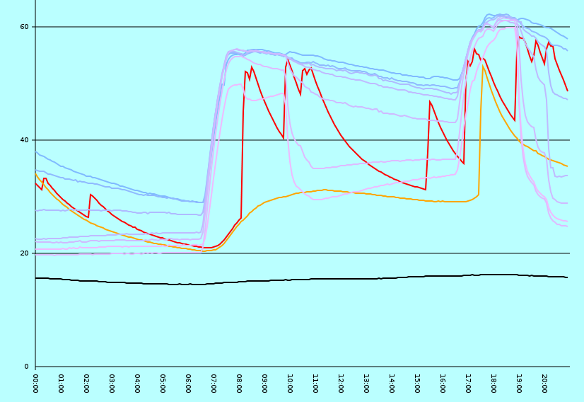
The graph to the left shows 21 hours worth of data, the key to the colours in the graph is
Loft Air above cylinder
Supply 1
Supply 2
Cylinder tapping 1
Cylinder tapping 2
Cylinder tapping 3
Cylinder tapping 4
Cylinder tapping 5
Cylinder tapping 6
Cylinder tapping 7
A few observations on the graph on the left:
When the boiler came on and started heating the hot water at 06:30, one can see the air temperature in the loft (the black line) start to raise, as the hot water cylinder started to heat the loft air space.
This data comes from a very wet May day in the UK, so ambient temperature influences would be lower than one might see on a sunny day.
The red and orange supply temperature lines (orange in particular) show a general lowering of the temperature in the supply pipes driven by the air temperature around the hot water cylinder (within the outer wrapping insulation), until the boiler started heating the hot water at 06:30, and then shows a gradual increase in the temperature driven by the increased air temperature around the cylinder.
Once a hot water supply is used, the respective supply probe temperature is quickly raised to that of the water leaving the top of the hot water cylinder, to drop back slowly again afterwards as the water in the pipe looses its heat to its surroundings again.
The seven blue through purple lines showing water cylinder temperatures for the first few hours of the day show the hotter water nearer the top of the cylinder cooling more rapidly than the cooler water lower down the cylinder.
The rapid heating of the water when the boiler started at 06:30 is shown by all seven cylinder probe temperatures rapidly climbing while the boiler was on, and then dropping back down, bottom of the cylinder first, as the red line shows hot water being used.
Most of the hot water was unused when the boiler kicked in again at 16:30, again raising all cylinder probe temperatures to about 60C, before more use of water is again seen bringing the various cylinder probe temperatures back down again.
The heat loss of the water in the cylinder is seen to be greater (a steeper line) in the blue lines to the right of the graph were the water temperature is higher than to the left of the graph where the water temperature is lower.